I recently attended a fascinating workshop on colonialism and its legacies organized by Jan Pierskalla. The substantive lessons of the workshop were many—including, for example, the challenges of maintaining law and order in Deutsch-Südwestafrika—but a common methodological theme that emerged is the problem of persistence. We may be able to identify variation within or across countries in colonial practices, laws, norms, settlement patterns, and so forth, but how can we link that to political phenomena decades or even centuries later? Why is it that colonial conditions have persistent effects even after colonialism is over?

One place where I have confronted this is in my work on colonial migration in Java and its effects on governance today (read here). It is easy to see why differences in Chinese settlement in 1930 would matter in 1930, but why would they matter today? A common argument underlying persistence is increasing returns, path dependence, or some kind of argument about spatial agglomeration. I made such an argument in the above-mentioned work. But there are two points to raise about this.

First, there is often a much simpler—if more boring—argument for persistence. Imagine two districts within a country, one that received a colonial treatment and one that did not. This might be high Chinese settlement (in my case above), or the mita (following Dell 2010), or something else altogether. If shocks to post-colonial politics are distributed randomly across the two districts, then those differences will persist for no other reason than initial conditions differed. How long? It depends on how frequent the shocks are and how widely they are applied. But this is an entirely coherent argument for what we might call real boring persistence.

We can show this visually. Below, we see two districts comprised of 10×10 units. The green one on the left is the “untreated” district. The blue one on the right is the “treated” district. Initially, the treatment is perfect: all cells are treated in the treated district, and none in the untreated district. 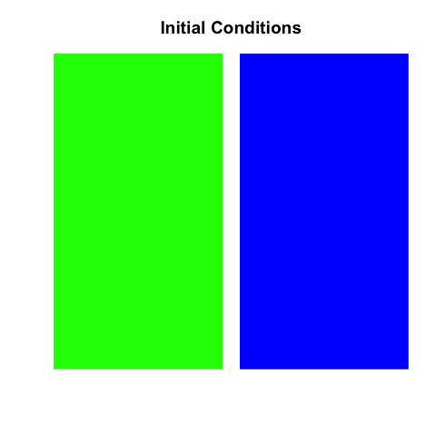Now let’s run history for one period. Let’s say that in each district, we’ll randomly choose ten units out of the one hundred there, and give them a 50% chance of switching. There’s no politics here, just randomness. If the units are, say, wells, and the periods are years, and the colonial legacy is differences is well availability, we can interpret this as saying that every year, for each of ten randomly chosen units there’s a 50% chance that a well is built (if there is no well there) or a well becomes unusable (if there is a well there). What do we get after one period? Something like this. 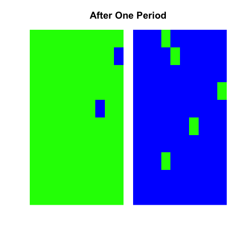We still see that the treated district is very different than the untreated district. But there’s no politics to this, it is purely a function of the initial conditions and the rate of well innovation or decay (here, 10%). Persistence is boring here, but it is real.

Now let’s run this history for fifty periods. What do we get? Something like this. 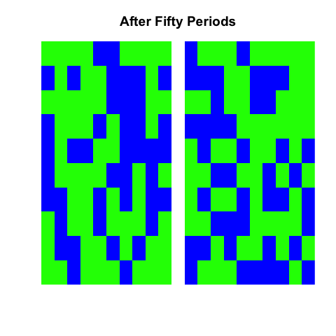After such a long history, there is no longer any difference between the two districts. We cannot tell which is which. We can inspect the history over each time period t to see how differences diminish. 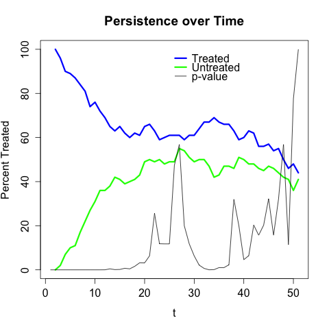The blue line here is the proportion of treated units in the originally treated district. The green line is the proportion of treated units in the originally untreated district. The black line is the p-value from a Fisher’s exact test that the two districts are different. We see here that it takes about twenty years (given the parameters above) for the two districts to become statistically indistinguishable from one another.

We of course can generate different results by changing the parameters. Let’s say that instead of a 50% chance of a unit changing from well to no-well or vice versa, it’s only a 10% chance. Then our history looks like this. 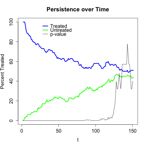It takes 120 years or so for the two to converge.

That, then, is the first point—that persistence may be real, but very boring. A second point is that one must be careful with arguments about increasing returns and path dependence. To see why, let’s imagine a different story of change. Let’s say that in each district, the number of wells that you have in year t is a function of the number of wells that you have in year t-1. Take first an extreme case in which the probability of wells appearing or disappearing is a simple function of the number of wells that you have: w/N, where w is the number of wells, and N is the number of units. The politics of such an argument are not material for my purposes here, but you might imagine a story in which districts with many wells find themselves better able to construct new ones or repair damaged ones than those with no or few wells. Now the probability that your well disappears is zero if all other units have wells in your district, the probability that a well is built is zero if you have no other wells in your district. In such a situation, persistence is infinite given the initial conditions above where w/N = 0 for the untreated district, and w/N = 1 in the treated district.

But imagine now a slightly more interesting situation. That is, the probability that you have a well is p = w/N + e, where e is a random shock in each period. Now, it is possible for a well to emerge in a district with no wells, and it is possible for a well to become unusable in a district with wells. Let’s plot such a situation, where e is drawn from a normal distribution with mean 0 and standard deviation 0.1. (A small technical note is that if w/N + e > 1 we will reset p = 1, and if w/N + e < 0 we will reset p = 0.) Here is what we get. 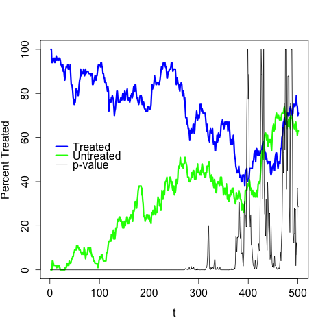It takes a long time for differences to disappear, because having wells increases your probability of having wells, and not having wells increases your probability of not having wells. But differences do indeed disappear around t = 375, and for some periods the two switch order. If I had given the distribution of e a larger standard deviation differences would have disappeared much more quickly.

The point of this slightly more interesting exercise is to suggest that phrases such as “increasing returns” and “path dependence” as justifications for persistence are tricky and demand care. The process above is one of state dependence (the probability of a well next year depends on the presence of a well today), but if there is any probabilistic element to the data at all, then state dependence implies only limited persistence. Modeling path dependence or increasing returns would be a more complex task. The takeaway, then, is that persistence can be very boring but easy, or it can be theoretical and hard. The places to look for more are Pierson (2000) and Page (2006), but I’d emphasize that these pieces are more often cited than they are read.