
Survey experiments are increasingly common in the social sciences, used to test causal claims using survey data where important features of survey questions can be randomized to see what effect this has on survey responses. Imagine something like this:
Many {Republican}{Democratic} candidates for office are worried about election integrity. How trustworthy do you think the upcoming midterm elections will be?
Survey respondents can get this question, some randomly assigned to get the version that includes {Republican}, and others the version that that includes {Democrat}. Comparing the distribution of answers to these questions across those two conditions allows us to estimate the effect of the Democratic versus Republican identity of the worrier on respondents’ views about election integrity, which might be an interesting question for some people.
As this methodology has become more established, survey designs have become more complicated. One important way that they have become more complicated is through what are called factorial experiments that vary more than one feature at the same time. Imagine such a question like this:
Many {Republican}{Democratic} candidates for office are worried about election {integrity}{fraud}. How trustworthy do you think the upcoming midterm elections will be?
Now there are two dimensions of variation, {Republican}{Democratic} and {integrity}{fraud}. This way we can estimate the effect of the partisan identity of the worrier, and also the effect of how we describe what they are worried about. These too might be interesting questions for some people.
One of the great benefit of experiments is that they are, ideally, very easy to analyze. A difference of means, or equivalently a linear regression with a dummy for treatment group, is a test of the null hypothesis of no difference between treatment states. But when it comes to factorial experiments, statistical analysis gets tricky. As I am working on a book chapter on survey experiments right now, I find myself reading a lot of contemporary survey experiments that use factorial designs. This led me to tweet the following yesterday:
To which Ben Lauderdale responded with the following:
Ben is noting that 2×2 factorial experiments are equivalent to conjoint experiments with two features that each have two levels. That has important implications that I have known about, but thinking through his reply convinced me that I didn’t really have an intuitive grasp of the stakes—and I suspect that I am not the only one. So rather than work on my book chapter,* I wrote the following post to help me understand the issue and explore the implications.
Backing Up: Conjoint Experiments
Conjoint experiments are also commonly used in political science, having been introduced and popularized by Hainmueller, Hopkins, and Yamamoto (2014). HHY also define, describe, and explain how to estimate a useful causal quantity known as the Average Marginal Component Effect (AMCE). This can be estimated using a regression with m-1 dummies for each of the m levels of a feature, for all f features. Conjoint experiments are frequently very complicated, with (say) f=7 features each with 2-4 possible levels, which is equivalent to (say) a 2x2x3x4x2x4x3 factorial experiment. But, if f=2 and m=2 for each, then a conjoint experiment is just like a 2×2 factorial experiment. HHY explicitly note this, writing
Finally, it is worth pointing out that the AMCE also arises as a natural causal estimand in any other randomized experiment involving more than one treatment component. The simplest example is the often-used “2×2 design,” where the experimental treatment consists of two dimensions each taking on two levels (e.g., Brader, Valentino, and Suhay 2008; see Section 1). In such experiments, it is commonplace to “collapse” the treatment groups into a smaller number of groups based on a single dimension of interest and compute the difference in the mean outcome values between the collapsed groups. By doing this calculation, the analyst is implicitly estimating the AMCE for the dimension of interest, where p(t) equals the assignment probabilities for the other treatment dimensions. Thus, the preceding discussion applies more broadly than to the specific context of conjoint analysis and should be kept in mind whenever treatment components are marginalized into a single dimension in the analysis.
This means that if you have a 2×2 factorial experiment you can estimate the AMCE via
…fitting a simple regression of the observed choice outcomes on the Dt-1 dummy variables for the attribute of interest and looking at the estimated coefficient for the treatment level
This, though, is not what I wrote in my tweet above. What’s going on?
Factorial Experiments, ATEs, and Interactions
To make sense of the difference, I turn to a working paper by Muralidharan, Romero, and Wuthrich (2022) which describes the challenges of estimating treatment effects in factorial experiments. They contrast two approaches for estimating the effects of variables T1 and T2 in a factorial experiment. The first is what they call the long regression:
Y = a + bT1 + cT2 + d(T1×T2)
The second is what they call the short regression:
Y = a + bT1 + cT2
The difference is clear: the long regression allows the effect of T1 to vary across values of T2, and the effect of T2 to vary across values of T1. The short regression does not; as MRW show, it implicitly assumes that there is no interaction between the effects of T1 and T2. If you knew that the effect of one treatment didn’t depend on the value of the other, you could use the short regression to estimate the Average Treatment Effect (ATE) of T1 and T2. If you did not know that, then estimating that regression could lead to biased estimates of those ATEs.
But if you look carefully, you will see that the short regression is equivalent to HHY’s linear regression estimator of the AMCE.
This observation helps to clear one thing up, which is that the ATE is not the same as the AMCE. The ATE is the difference in outcomes between treatment states. The AMCE has a slightly woolier definition: it is the
marginal effect of attribute l averaged over the joint distribution of the remaining attributes
That is generally a useful thing to know! But it is not the same as the ATE.
AMEs versus AMCEs
That much I knew prior to Ben’s reply to my tweet. What I didn’t quite understand, though, was how this difference mattered and why. Others might see the implications of this distinction immediately, but I can only make sense of these things by exploring some homemade data to see how these estimators fare “in the wild.” Well, if I must, I must.
To do this, I put together a little simulation of a 2×2 factorial experiment. This allows me to vary the effects of T1 and T2 and also to explore what happens if the effect of one depends on the value of the other. I can also compare estimates of various causal effects obtained via various statistical procedures. For simplicity, I look only at the effects of T2, although this all generalizes to T1. I will focus on three estimated causal effects.
- The AMCE of T2, estimated via the short regression
- The ATE of T2, estimated via the long regression (but varying across values of T1, so there are two distinct ATEs).
- The average marginal effect (AME) of T2, derived from the long regression.
What’s this AME? It is the difference in the predicted values when T2=0 and T2=1, averaging over all of the values of T1. Although this is not precisely correct, it may be thought of as the average of the ATE of T2 when T1=0 and the ATE of T2 when T1=1,. As we will see, sometimes the AME is the same as the AMCE, but it is not always so.
To illustrate this, see this little simulation exercise. The idea is, generate some known effects of T1 and T2 and then see if you can recover them from various regression models. This code will do this (using the margins package which allows R to ape Stata’s margins command):
simulate_shortlong <- function(n1,n2,p1,p2,a,b,c,d) {
y_out <- c(rep(a,n1*p1),rep(b,n1*(1-p1)),rep(c,n2*p2),rep(d,n2*(1-p2)))
t1 <- c(rep(0,n1),rep(1,n2))
t2 <- c(rep(0,n1*p1),rep(1,n1*(1-p1)),rep(0,n2*p2),rep(1,n2*(1-p2)))
y <- y_out + rnorm((n1+n2),0,5)
short <- lm(y ~ t1+t2)
long <- lm(y ~ t1*t2)
out.short <- margins_summary(short, variables="t2")
out.long <- margins_summary(long, variables="t2")
return(data.frame(c(out.short[2], out.long[2],
margins_summary(long, variables="t2", at=list(t1=0:1))[1,3],
margins_summary(long, variables="t2", at=list(t1=0:1))[2,3],
out.short[5],
out.long[5])))
}
You’ll see we have the parameters a, b, c, and d which correspond to Y00, Y01, Y10, and Y11, the outcomes under the two possible values (0,1) that T1 and T2 can take. Then there is some error, set so that we explain roughly 20% of the variation in Y via the two treatments. We also have four additional parameters: n1, n2, p1, and p2. The first two give you the proportion of units getting T1 and T2, and the latter two are the proportion of each that get the treatment condition. So if n1 = n2 = 500, and p1 = p2 = .5, there are 1000 total observations (n1 + n2), and half of each get treated by each variable, for 250 observations in the 2×2 factorial experiment.
(The reason I am telling you all this now is because it will matter later.)
Let’s try that experimental design, with a = 0, b = 0, c = 0, and d = 1, replicating this analysis 100 times. Here, ATE of T2 = 0 when T1 = 0, and 1 when T1 = 1. The AME is the average of those: 0.5.
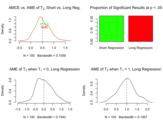
The upper left hand plot contains both the AMCE estimated from the short regression and the AME estimated from the long regression. The two density plots are exactly the same, which is good; and centered around the correct AME. Now, as the bottom two figures show, the long regression also allows you to estimate the ATEs correctly for both values of T1, but if you stipulated that you did not care about that all, you would be pleased to know that the AMCE and the AME are the same. You could use either the short regression to estimate the AMCE, or the long regression to estimate the AME, but they estimate the same thing.
But what if we don’t have such a perfect distribution of treatments with equally sized cells in the 2×2? Let’s see what happens.
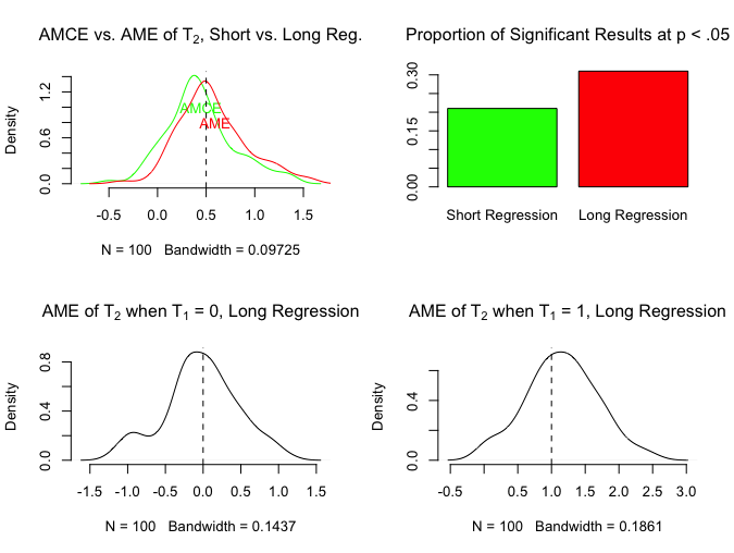
Now the AMCE estimated from the short regression and the AME calculated from the long regression are not the same. The AME continues to correctly estimate the average of the two ATEs, but the AMCE estimates the effect of T2 averaged over the distribution of treatment conditions, which is no longer equal. That is what the AMCE is supposed to do (that’s what the pull-quote above that defined the AMCE was saying), so nothing wrong with that per se.
We can get similar results by varying the distribution of T1 but keeping the distribution of T2 equal across the values of T1.
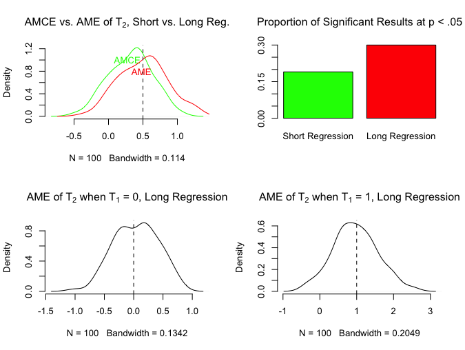
Same basic result as in the previous example: the AME is correctly estimated from the long regression, and it is no longer the same as the AMCE estimated from the short regression.
To close out the discussion, let’s take a more extreme case in which the ATE of T2 is -2 when T1 = 0, and 2 when T1 = 1. So T2 has positive effects or negative effects depending on whether it was assigned 0 or 1 from T1, and they perfectly cancel out. As a result, the AME should be 0. What happens?
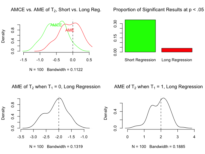
Here is a situation where if you actually cared to estimate the AME of T2 (and were uninterested in heterogeneity of the ATE of T2 across values of T1), you would conclude something very different based on the short versus long regression. The short regression gives you an AMCE of T2 that is often negative and statistically significant, whereas the long regression gives you an AME of 0 (and fails to reject the null that it is 0).
Summing Up
Working through these examples helps to develop intuitions about what the AMCE corresponds to, and its value when analyzing 2×2 (or other) factorial experiments. Here are the main takeaways:
- The point of my original tweet stands. If you have conducted a 2×2 factorial experiment, you should estimate the long regression and look for heterogeneity in the ATEs of the two treatment arms. All of the reasons that MRW give in favor of doing it this way hold.
- If you actually do not care about that heterogeneity, and are only interested in the effect of one treatment arm unconditional on the other, you should still estimate the long regression and calculate the AME from that. There’s no excuse not to do that, thanks to
margins. - If you know that your sample has equal numbers of observations in each of the four cells of the 2×2, and you only care about the AME, only then should you estimate the short regression, because here the AMCE and the AME will coincide and it won’t matter.**
- One could in principle be interested in the AMCE itself in a 2×2 factorial experiment. For example, perhaps the joint distribution of treatment states was assigned to be imbalanced on purpose, in a way that represented some feature of the real world. In this case, the AMCE could be a quantity that is useful for some sort of claim about external validity. (That said, I am not aware of any factorial experiment designed in such a way that the AMCE was a causal quantity of interest in this regard.)
- This recommendations do not have any direct implications for HHY’s analysis of conjoints and the utility of estimating AMCEs from them. First, it remains the case that AMEs and various subgroup ATEs are likely not estimable when there are large numbers of potential combinations of profiles. Second, as HHY note, if one were interested in a particular subset of these interactive effects, they could be estimated from conjoint data too—although not via the short regression, but rather by carefully specifying a different regression. See, e.g., Egami and Imai (pdf) on Average Marginal Interaction Effects.
NOTES
* Sorry John.
** I do not know if this holds when adjusting for pre-treatment covariates that might be imbalanced across treatment arms.
