Category: Uncategorized

I have found myself thinking a lot recently about multiple imputation in the presence of colliders. Proponents of MI commonly recommend that any variable available in the dataset should be included in the imputation stage, even if it will not be included in the analysis stage. In one important statement (PDF):

For greater efficiency, add any other variables in the data set that would help predict the missing values (p. 57).

I have often wondered if this is true—if there are particular cases in which adding variables atheoretically at the imputation stage can lead to bias in the analysis stage even if the analysis stage model is correct.

Colliders are a candidate for such a variable. A collider is a variable that is jointly caused by both an independent variable and a dependent variable: X -> C <- Y. It is well-known that in a regression of Y on X in which the true causal effect of X is zero, conditioning on a collider can create the illusion that X actually causes Y. Take the simple case where X and Y are random variables that are unrelated to one another, but imagine that they jointly cause a third variable C, and we include that as a control variable. If we were to generate those data and run that regression in R, here is what we would get.

x <- rnorm(100)
y <- rnorm(100)
c <- y + x + rnorm(100)
summary(lm(y~x+c))$coefficients

##               Estimate Std. Error   t value     Pr(>|t|)
## (Intercept)  0.1009087 0.07196625  1.402167 1.640576e-01
## x           -0.3802116 0.09452905 -4.022166 1.141927e-04
## c            0.4776374 0.04893261  9.761127 4.397550e-16

Conditioning on a collider in this simple example generates a highly significant but entirely spurious correlation between X and Y.

So what happens if you were to include a collider when imputing missing data? My intuition is that doing so would create similar problems, but to test that intuition I made a little simulation.* Consider the best possible case: the analyst knows that the correct analysis model excludes the collider, but includes the collider in the imputation stage because it is correlated with the variables with missing data. First load the necessary packages and reset ggplot2's colors away from the default mouldy waffle setting.

library(mice)
library(reshape2)
library(ggplot2)
theme_set(theme_classic())
set.seed(14850)

The following function simulates a dataset with missing data in Y those probability of missingness depends on the value of Y. It then runs five analyses

1. with the full data (no missing values): Full
2. using listwise deletion/complete case analysis: LD
3. using MI using no auxiliary variables: MI
4. using MI but with a proxy variable for Y: MI-full
5. using MI but with the collider C: MI-collider

simulation<-function(p){

  # set up the data 
  N <- 1000
  x <- rnorm(N)
  u.y <- rnorm(N)
  y <- u.y + rnorm(N)
  c <- y + x + rnorm(N)

  # full data frame, no missing values
  dat.full <- as.data.frame(cbind(y,x,u.y,c)) 

  # create missingness in Y
  dat.missing.collider <- dat.full                     
  dat.missing.collider$miss.y<-rbinom(N,1,pnorm(y+p))
  dat.missing.collider$y[dat.missing.collider$miss.y==1]<-NA
  dat.missing.collider$miss.y <-NULL  

  # df includes Uy but no collider, missing values for Y
  dat.missing.full<-dat.missing.collider
  dat.missing.full$c<-NULL

  # df includes collider but not Uy, missing values for Y
  dat.missing.collider$u.y <- NULL    

  # df omits Uy and c, missing values for Y
  dat.missing <- dat.missing.collider
  dat.missing$c <- NULL                 

  # if all data were observed
  res.full <- summary(lm(y ~ x, data=dat.full))$coefficients
  b.full <- res.full[2,1]
  p.full <- res.full[2,4]

  # listwise deletion
  res.missing.ld <- summary(lm(y ~ x, data=dat.missing))$coefficients
  b.missing.ld <- res.missing.ld[2,1]
  p.missing.ld <- res.missing.ld[2,4]

  # impute the data
  mi <- mice(dat.missing)                   
  mi.full <- mice(dat.missing.full)          
  mi.collider <- mice(dat.missing.collider) 

  # results without c or Ux, Uy
  res.missing.mi <- summary(pool(with(mi, lm(y ~ x))))
  b.missing.mi <- res.missing.mi[2,1]
  p.missing.mi <- res.missing.mi[2,5]

  # results with Ux, Uy
  res.missing.mi.full <- summary(pool(with(mi.full, lm(y ~ x))))
  b.missing.mi.full <- res.missing.mi.full[2,1]
  p.missing.mi.full <- res.missing.mi.full[2,5]

  # results with collider
  res.missing.mi.collider <- summary(pool(with(mi.collider, lm(y ~ x))))
  b.missing.mi.collider <- res.missing.mi.collider[2,1]
  p.missing.mi.collider <- res.missing.mi.collider[2,5]

  outputs <- cbind(b.full,
                   b.missing.ld,
                   b.missing.mi,
                   b.missing.mi.full,
                   b.missing.mi.collider,
                   p.full,
                   p.missing.ld,
                   p.missing.mi,
                   p.missing.mi.full,
                   p.missing.mi.collider)
  return(outputs)
}

Run this simulation 250 times and collect the output.

sims <- data.frame(t(matrix(replicate(250, simulation(0)),nrow=10)))
sims <- cbind(1:nrow(sims),sims)
names(sims) <- c("Iter",rep(c("Full","LD","MI","MI-full","MI-collider"),2))

First, we compare the estimates across all five estimators (remembering that the true effect of X on Y is zero).

colMeans(sims[2:6])

##         Full           LD           MI      MI-full  MI-collider 
## 0.0006753861 0.0030361351 0.0016691195 0.0021527321 0.0029543371

to.plot.b <- melt(sims[1:6], id.vars="Iter", variable.name="Estimator", value.name="Estimate")
ggplot(to.plot.b, aes(x=Estimate, color=Estimator)) + geom_density()

This looks pretty good: the distribution of coefficient estimates is centered around zero for each of these models, and the mean results for MI with a collider aren't any worse than for MI without a collider. But what of Type-1 error rates, a particular concern when conditioning on a collider?

colMeans(sims[7:11]<.05)

##        Full          LD          MI     MI-full MI-collider 
##       0.044       0.060       0.036       0.048       0.044

To my surprise, Type-1 error rates don't seem to be a problem here so long as the collider does not appear in the analysis stage.

Puzzled by this result and not believing my lying eyes, I looked online for further discussion, and came across this interesting paper (PDF) on auxiliary variables in MI. They diagnose a more subtle problem: sometimes adding a collider into the imputation stage can transform the data missingness from Missing at Random (MAR) to Missing Not at Random (MNAR). In the simulations above, data are MAR because they were confined to Y and we have X through which to model Y. But if Y causes a variable C that is correlated with the missingness mechanism and that missingness mechanism also depends on X, then conditioning on C will transform MAR data into MNAR data.

To illustrate this problem, adjust the simulation function as follows:

simulation_coll_missingness<-function(p){

  # set up the data 
  N <- 1000
  u.y <- rnorm(N)
  u.c <- rnorm(N)
  x <- rnorm(N)
  y <- u.y + rnorm(N)
  c <- y + u.c + rnorm(N)

  # full data frame, no missing values
  dat.full <- as.data.frame(cbind(y,x,u.y,c)) 

  # create missingness
  # p(Y missing) correlated with C and X
  dat.missing.collider <- dat.full                     
  dat.missing.collider$miss.y<-rbinom(N,1,pnorm(u.c+x)) 
  dat.missing.collider$y[dat.missing.collider$miss.y==1]<-NA
  dat.missing.collider$miss.y <-NULL  

  # df includes Uy but no collider, missing values for Y
  dat.missing.full<-dat.missing.collider
  dat.missing.full$c<-NULL

  # df includes collider but not Uy, missing values for Y
  dat.missing.collider$u.y <- NULL    

  # df omits Uy and c, missing values for Y
  dat.missing <- dat.missing.collider
  dat.missing$c <- NULL                 

  # if all data were observed
  res.full <- summary(lm(y ~ x, data=dat.full))$coefficients
  b.full <- res.full[2,1]
  p.full <- res.full[2,4]

  # listwise deletion
  res.missing.ld <- summary(lm(y ~ x, data=dat.missing))$coefficients
  b.missing.ld <- res.missing.ld[2,1]
  p.missing.ld <- res.missing.ld[2,4]

  # impute the data
  mi <- mice(dat.missing)                   
  mi.full <- mice(dat.missing.full)         
  mi.collider <- mice(dat.missing.collider) 

  # results without c or Ux, Uy
  res.missing.mi <- summary(pool(with(mi, lm(y ~ x))))
  b.missing.mi <- res.missing.mi[2,1]
  p.missing.mi <- res.missing.mi[2,5]

  # results with Ux, Uy
  res.missing.mi.full <- summary(pool(with(mi.full, lm(y ~ x))))
  b.missing.mi.full <- res.missing.mi.full[2,1]
  p.missing.mi.full <- res.missing.mi.full[2,5]

  # results with collider
  res.missing.mi.collider <- summary(pool(with(mi.collider, lm(y ~ x))))
  b.missing.mi.collider <- res.missing.mi.collider[2,1]
  p.missing.mi.collider <- res.missing.mi.collider[2,5]

  outputs <- cbind(b.full,
                   b.missing.ld,
                   b.missing.mi,
                   b.missing.mi.full,
                   b.missing.mi.collider,
                   p.full,
                   p.missing.ld,
                   p.missing.mi,
                   p.missing.mi.full,
                   p.missing.mi.collider)
  return(outputs)
}

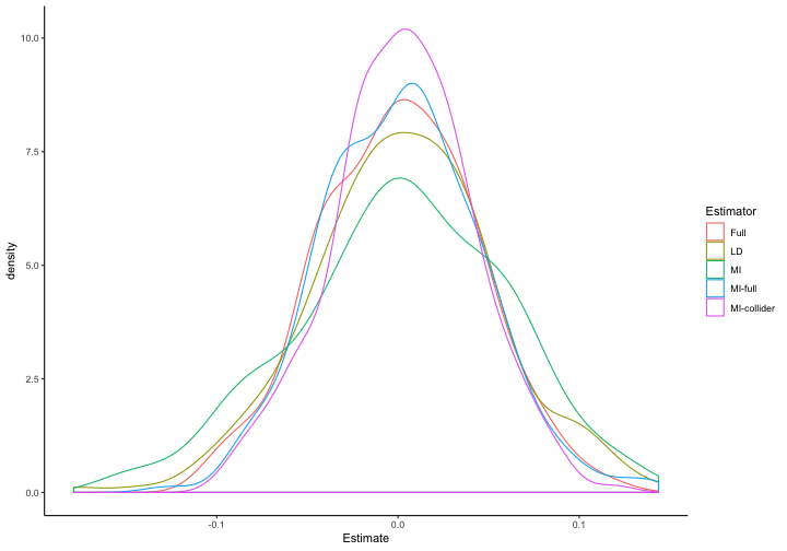
The difference is now that the probability that Y is missing depends both on a factor that determines C and on X. Simulating these data 250 times again, here is what we get:

sims <- data.frame(t(matrix(replicate(250, simulation_coll_missingness(0)),nrow=10)))
sims <- cbind(1:nrow(sims),sims)
names(sims) <- c("Iter",rep(c("Full","LD","MI","MI-full","MI-collider"),2))
to.plot.b <- melt(sims[1:6], id.vars="Iter", variable.name="Estimator", value.name="Estimate")
ggplot(to.plot.b, aes(x=Estimate, color=Estimator)) + geom_density()

Now we see that using a collider in the imputation stage generates bias in the analysis stage even when the analysis stage does not control for the collider.

colMeans(sims[7:11]<.05)

##        Full          LD          MI     MI-full MI-collider 
##       0.028       0.040       0.048       0.052       0.644

And Type-1 error rates are unacceptably high.

What is an example of an “imputation-stage collider”? Imagine we wish to use education (X) to predict partisanship (Y), but we have missing data on partisanship for people who feel excluded from the political system and who also have lower levels of education. And let's also imagine that members of party R are more likely to respond that they don't trust the government (C), as are people who feel excluded from the political system. Adding trust in government at the imputation stage will bias estimates of the effect of education on partisanship, but excluding it (given a series of other assumptions about what causes what that I'll leave unspecified here) would not.

Note also that trust in government should be highly correlated both with education and with partisanship, so it looks like a good candidate for including in our imputation model if all we thought about was its predictive capacity.

So what have we learned from this exercise? The main takeaway—as always—is that for MI to yield unbiased estimates of regression coefficients or causal parameters of interest, its assumptions have to be met. But more precisely, even having the correct model of the analysis stage does not absolve the analyst of considering the relationship between the imputation stage variables, the causal model, and the missingness mechanism. It turns out that in this simple example, imputing with an analysis-stage collider is innocuous (so long as it is excluded at the analysis stage). But imputation-stage colliders can wreck MI even if they are excluded from the analysis stage.**

As I have argued elsewhere, MI cannot be a theory-free exercise. Just as there is no rule of thumb for comparing MI to its alternatives, there is no simple rule of thumb for auxiliary variables such as “include as many variables as you can in the imputation stage” or “in principle, including all of the remaining auxiliary variables in the imputation model is desirable” (PDF).

NOTES

*This post also serves as a test to see if I could make the Rmarkdown-to-Wordpress integration work, via knit2wp.
**And in case you're wondering if including the imputation-stage collider as a control in the analysis stage will help, it won't.

On Wednesday, Indonesia will have elections for its president, legislature, and hundreds of regional governments. For watchers of religion and politics, national elections are always an opportunity for reflection on the apparent rise of Islam as a political force in Indonesian democracy. And yet the role of Islam in this country of 230 million Muslims (and 30 million-plus non-Muslims) is complicated, as much a statement about identity as it is a statement about religious observance or conservatism. This distinction is essential for making sense of Islam as a political force in Indonesia, and has lessons that travel to other contemporary democracies in plural societies.

What does it mean to conceptualize Islam as identity politics? Put plainly, it means that voters and citizens conceptualize politics in terms of people who share ascriptive characteristics with them. Identity is multidimensional—we all have many identities, some of which are more salient than others, and this salience can vary across social situations, as Judith Nagata showed in her landmark study of ethnicity in Malaysia. But in Indonesia, religious identity is one of a few dimensions of identity that is highly salient across social situations. One might vote for, or support the actions of, a politician who appeals to one’s shared religious identity. With a population that is nearly 90% Muslim, no credible presidential candidate can win office without the support of Muslims.

Contrast this to a conceptualization of Islam and politics that focuses on religiosity, piety, or conservatism. Here, politicians earn support through their religious credentials, their personal piety, or their ability to pass religious regulations. The past two decades of Indonesian democracy have seen the rise of a more conspicuous and expressive form of Islam,* more visible in everyday life in the form of dress and manner of speech as well as in religious observance. But there is scant evidence that expressive Islam corresponds to religious politics. It may, instead, be that expressive piety is a form of identity maintenance in the face of the complex changes associated with modernization, urbanization, and social change experienced by Indonesia’s Muslim population.

Islam-as-identity has very different implications for Indonesian politics than does Islam-as-religiosity. The former emphasizes the construction of Indonesian politics in terms of the status of groups and their representation by politicians qua groups. The latter emphasizes politicians’ religious character. The strategy for a politician running in an Islam-as-identity world is to establish that s/he looks like a Muslim candidate; the content of the candidate’s platform or his/her religious behavior does not much matter. And in a world in which Islam-as-identity dominates, a winning strategy to appeal to Muslim voters who are happy with the performance of a non-Muslim incumbent is to simply claim that Muslims must not vote for non-Muslims, as Liam Gammon and Eve Warburton showed in the April 2017 Jakarta gubernatorial election.

Such debates are visible today, in a contest pitting one Javanese Muslim versus another Javanese Muslim. On one hand, President Joko Widodo attempts to show his religious credentials. On the other hand, his opponents allege that he is a Christian. It is the latter that has more resonance than any commentary about how seriously he practices his faith, especially since neither Prabowo Subianto nor Sandiaga Uno have any particular reputation for religious piety themselves.** Instead, what they have is endorsements from Islamic parties and Islamists. That suffices to license them as “Muslim” candidates. Jokowi’s choice of an influential Muslim religious leader as his running mate, on the other hand, shores up concerns that he is a “Muslim” candidate too.

The lesson from Indonesian democracy is even though the “rise of Islam”*** may mean a more expressive form of Islam in public life, it also may harden political cleavages that are not, at root, about religiosity or conservatism. What might counteract this process? In the Netherlands, which had been characterized by “the politics of accommodation” among Protestants, Catholics, and seculars through the 1970s, the decline of religious observance undermined identity-based political competition. That does not seem likely in the near future in Indonesia.

The lessons of Islam and identity in Indonesian politics travel to other plural societies. Mayor Pete may be a more observant Christian than President Trump, but this does not much matter if he does not represent the social category of “Christian.” And President Trumps awkward relationship with the details of his professed faith may not matter if he does fit that category. There is no illogic here. The evidence of President Trump’s identity as a Christian is the fact that Christian elites endorse him. That they do so on the intuition that they will be able to shape his agenda in ways consistent with their Christian values reveals the indirect ways that religion-as-identity may be exploited by those who actually do care about religion-as-conservatism.

So, too, in Indonesia.

NOTES

* This “Islamic turn,” however, preceded Indonesian democracy: see Hefner, Liddle, and the works of Indonesian Muslim thinkers like Cak Nur and Amien Rais.
** Sandi, however, is trying to build one.
*** I am not so certain that Islam is actually “rising” in Indonesia, but for the purposes of this discussion I proceed as if this were true.