A recent post at New Mandala asks how bad is Thaksinomics, the suite of policies associated with Thailand’s former Prime Minister Thaksin Shinawatra and the parties and movements which have succeeded him. The post contains some nice illustrative data but struggles to be convincing because it leaves unspecified the question of how bad compared to what?
Being exact about the benchmarks for evaluating Thaksinomics is hard. But it is necessary for the data to be meaningful, or even for the question to be coherent. The only explicit comparison that we see is Thailand’s economic growth compared to Australia’s, but this isn’t too revealing: Australia’s higher GDP per capita means that we should expect it to grow more slowly than Thailand, as any textbook in modern economic growth will show.
To make headway on this question, we need to find some way to compare Thailand with some kind of Thailand that didn’t have Thaksin as PM from 2001-6. Here we see the fundamental problem of causal inference, because it’s impossible to do this. We cannot observe Thailand without Thaksin.
A recent approach pioneered by Alberto Abadie, Alexis Diamond, and Jens Hainmueller (forthcoming AJPS, ungated here) offers a structured way to think about how to answer such questions. The intuition is that we should look for some country which is a good comparison for Thailand—following the same strategy that motivates the Australia comparison—but that we can use a weighted average of other countries’ experiences to provide an estimate of what Thailand would have looked like from 2001 until today rather than any one country.
Like the New Mandala post, let’s focus on GDP growth. The procedure is that we (1) specify the determinants of GDP growth, (2) find the weighted average of countries that best matches Thailand’s record of GDP growth prior to 2001, (3) use those weights in combination with the determinants of GDP growth to simulate a path of GDP growth after 2001. Maria Wihardja and I recently applied this methodology to understand the effects of Indonesia’s decentralization (gated, ungated PDF), and it offers one way of confronting the fundamental problem of causal inference for macro-level policy changes.
We can do this very easily (the R code is here). Let’s specify the predictors of GDP growth to be log of GDP, population, economic openness, investment as a share of GDP, and level of democracy. We’ll look at 1980-2010, and set 2001 at the treatment year. We’ll also specify that the synthetic control country should match Thailand in 1980 (onset of the analysis window), 1990 (prior to the 1990s boom), 1996 (prior to the Asian Financial Crisis), and 1998 (at the depth of the crisis). Here is what we find.
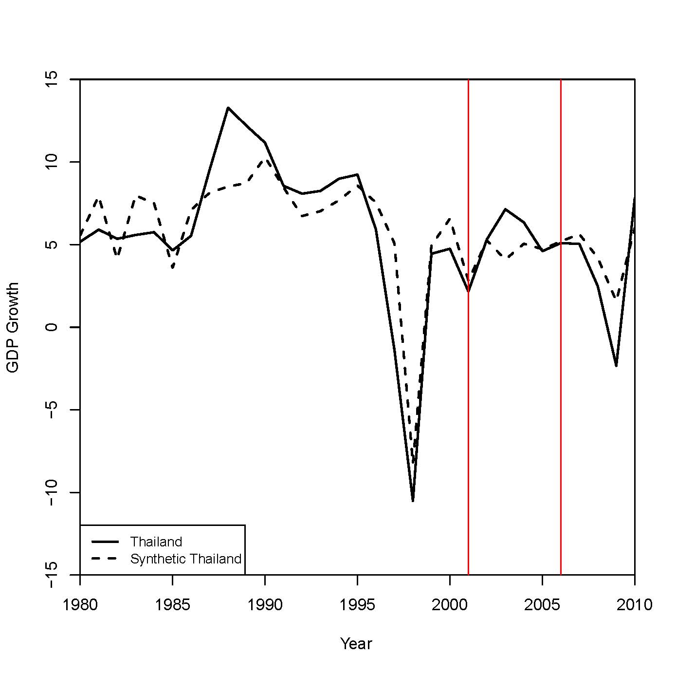
The red lines correspond to 2001 (Thaksin elected) and 2006 (Thaksin ousted). We can see that Thailand actually did do better than our best prediction of what Thailand’s growth would have been between 2001 and 2006. We also see that the pattern reverses after 2006. In case you’re curious, the weighting matrix has positive weights for Indonesia (.363), South Korea (.321), Malaysia (.212), and Swaziland (.102). Our best guess of the effect of Thaksin on economic growth is positive between 2001 and 2006, but that it turned negative afterwards. One possible interpretation is that the country’s ongoing political crisis since the 2006 coup has overwhelmed whatever benefits Thaksinomics might have brought.
This analysis makes a lot of assumptions. However, the benefit of such an analysis is that these assumptions are clear, they are reproducible, and they are contestable: if you disagree, you can show me how different assumptions lead to different conclusions.