Category: Research

A recent post at Duck of Minerva by Peter Henne raised the question of multiple comparisons in international relations research. He poses the problem like this:

Imagine we’re writing a paper on interstate conflict. We could measure conflict onset, duration or intensity. We could measure intensity by an ordinal scale, the number of deaths, or other more complicated measures. We could include all dyads, politically-relevant dyads, dyads since 1945, 1989, etc. Ideally these choices would be based on our theory, but our theories are often not specific enough to specify such choices.

I find this striking, because even though the post is about “what the ‘multiple comparisons issue’ really is,” this is not how I customarily think of multiple comparisons. The above description captures a problem of uncertainty and/or researcher discretion in measurement of one variable. Yet most overviews of the multiple comparison problem describe the problem of uncertainty and/or researcher discretion in choosing what outcome to measure or measuring multiple outcomes.

The difference is subtle but important. Let’s take an example of the democratic peace in international relations. Imagine a well-designed (if implausible) experiment that randomly assigns half the world’s countries to be democracies. We then look for the consequences. We might be interested in the effect of democracy on war, but be uncertain in how to measure it. A continuous measure of people killed in conflict? A binary measure that is 1 if the conflict reaches some intensity, zero otherwise? An ordinal scale of none-some-lots of war? Maybe our measures of people killed are biased? Maybe we have many such measures, each biased in a different but unknown way? We might try to use all of them as dependent variables to see how inferences change. That is uncertainty in measurement of one variable. If we report only the ones that statistically significant results, then we have researcher discretion in the same.

The multiple comparison problem, however, often describes something different. This is when we look for all sorts of outcomes of the experiment. Not just war (however measured) but also economic growth. Or tax collection. Or social rights. Or environmentalism. Or religiosity. Or any number of things. Maybe we try all of them as dependent variables to see what the experiment affected. That is uncertainty in choosing what outcome to measure. If we only report the ones that produced statistically significant results, then we have researcher discretion in the same.

The problem with the latter is that if you keep picking dependent variables, you will eventually find one that is correlated with the treatment just by chance. One might then infer that the treatment affected that outcome. We can address this problem by adjusting the target level of statistical significance required to draw inferences about the treatment, increasing the “standard” for statistical significance to correct for the fact that one has looked for many outcomes. That is one solution to the multiple comparisons problem. Another is pre-registration.*

Does it matter if the dependent variables are multiple measures of the same thing versus multiple different dependent variables? My intuitions suggest that the answer is yes, but I could not figure out how, and this masterful review of the multiple comparisons problem does not distinguish between the two except for indirectly, in the case of the dependent variables being correlated with one another (in other words, the tests are not independent). So to get a handle on this, I created a little simulation that compares two types of analyses. I created a binary treatment variable T, and then correlated it with some randomly created dependent variables.

1. In the first, there are twenty dependent variables that measure different things. I simulated these with twenty randomly generated dependent variables Y1,Y2,…,Y20.
2. In the second, there are twenty different measures of a single dependent variable Y. One is Y itself. Another is a dichotomized version of Y. Still another is Y measured as an ordinal variable. Some others are Y variables plus some non-random noise. And so forth—some measures are closer to Y than others, some are dichotomous or ordinal variables. I got pretty creative here. The idea is that this reflects uncertainty in measurement of a single dependent variable.

Importantly, each of these dependent variables was generated independently of T. So we know that the experiment did not cause any outcome. But if we were to select a standard of statistical significant of 95%, we would find that 5 out of every 100 random dependent variables would be correlated with the T entirely by chance. Or, in this case, 1 out of the 20 that I created for the first analysis. And there would only be a 5% chance that the single dependent variable $Y$ would be associated with that treatment variable in the second analysis. Any statistically significant correlation between the treatment variable and any dependent variable is therefore a false positive.

I then simulated these analyses 500 times, for random draws of the treatment variable and the DVs. For each, I calculated how many false positives showed up in each analysis of the twenty dependent variables (which I’ll call the “Many DVs” scenario) and how many false positives showed up in each analysis of the twenty measures of the single dependent variable (“One DV, Many Measures”).** The figure below compares the results.

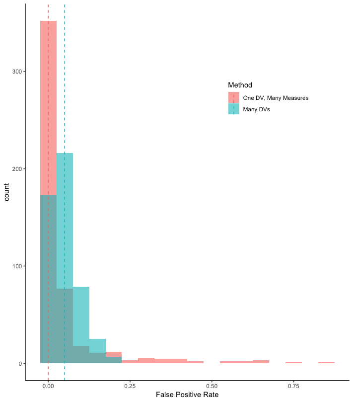
The histograms show the distribution of false positives. The dotted lines are the median false positive rate across the 500 simulations. These results are quite revealing.

1. In the the “Many DVs” scenario, as expected, the modal outcome is that 1/20 or .05 of the results are significant at the 95% confidence level. This is as expected in the multiple comparisons literature.
2. In the “One DV, Many Measures”, results are very different. The most common outcome is that no results are significant. But when they are significant, they are much more likely to be significant across many measures. That is the long right tail of that distribution.

These differences help to clarify what the problem of multiple comparisons is and also how corrections for it might or might not work. Multiple tests of the same dependent variable measured differently might not increase our confidence in the result if they are all due to the chance of that DV, because they are not independent tests. A multiple comparison adjustment will decrease the false positive rate in the “One DV, Many Measures” scenario, but this is a mechanical result, one that comes from just increasing the threshold for statistical significance.

By contrast, in the “Many DVs” scenario, adjustments for multiple comparisons respond directly to the fact that too many independent tests will eventually yield significant results simply by chance.

NOTES

* Although in principle, one might also pre-register a fishing expedition (which my colleagues and I once termed “hypothesis trolling” or “hypothesis squatting”).

** I used logits and ordered logits where appropriate in the “One DV, Many Measures” tests.

As part of a series of ongoing projects on migration and populism (see e.g. here), I happened to come across a report from the 2010 Japanese Census. It contains data on Japan’s foreign population since 1950, and how it has changed. A couple of quick plots of these data are remarkably revealing.

First, look at the changes in numbers. Japan’s population was well under 1% foreign until the 1980s, when you see a large jump corresponding to the post-oil crisis reforms to Japanese citizenship laws and continuing into the Lost Decade.

At the same time, the sex ratio basically flips, but gradually rather than discontinuously with the 1980s reforms. The sex ratio among foreigners living in Japan was basically 1.2 men for every woman in 1950, and it is now closer to 0.8 men for every woman.

Who are these foreigners? We can break out the trends by nationality:

For most of the twentieth century, Koreans have comprised by far the largest population of foreigners in Japan. That proportion declined precipitously in the 1980s, as a result of two processes. First, the above-mentioned citizenship reforms. But second, the gradual naturalization of Japanese of Korean descent (previously counted among the foreigners). So this reversal is partially due to higher relative immigration by non-Koreans, and partially due to composition effects. What is most striking is the increase in “Others,” comprised partially of Brazilians and Peruvians (the dekasegi) but also Southeast and South Asians.

Japan still has a far smaller immigrant population than nearly all other OECD countries. But Japan is no longer the mono-ethnic society, closed to foreigners, that it once was. But unlike the initial years of labor migration into Western Europe after WWII, women rather than men are leading the way. That is interesting, and it probably will have political consequences.